I wrote in a previous blog post about the different components of RAG and why there are three scores that we need to pay attention, in this one I want to zoom on the retriever itself and document the eight metrics used to score it on its own. I will reuse the same example again.
The knowledge base has 10,000 chunks. For "What is our refund policy when a parcel is marked delivered but the customer says it never arrived?", exactly 6 of them are relevant. The retriever returns its top 5: the returns policy, the disputed-delivery SOP, the holiday schedule, the carrier liability clause, and a delivery-delays FAQ. Two of the five are relevant.
The accuracy trap
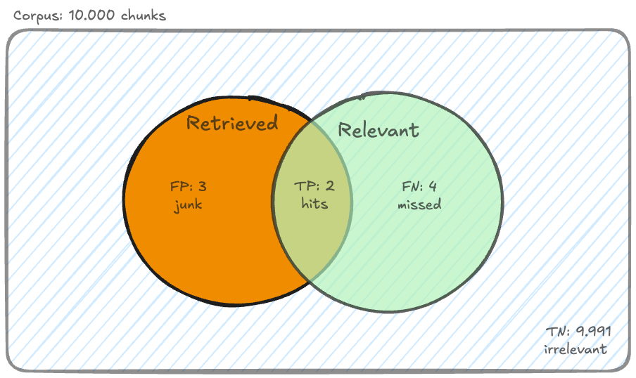
Accuracy counts correct decisions over all documents: the relevant ones you retrieved (true positives) plus the irrelevant ones you correctly left in the index (true negatives).
For our query: TP = 2, FP = 3, FN = 4, and TN = 9,991, because the retriever correctly did not retrieve 9,991 irrelevant chunks.
That last number is the trap. . The retriever missed two thirds of the relevant documents and ranked an irrelevant one first, and accuracy calls it near perfect.
In a large corpus almost everything is irrelevant to any given query, so the true negatives drown the signal. Accuracy is the first metric in every textbook and the last one you should use for retrieval.
Precision and recall
Precision is quality: of what was retrieved, how much was relevant.
In practice 0.40 means three of the five chunks the generator must read are junk: the returns policy, the holiday schedule, and a delays FAQ.
Recall is coverage: of everything relevant, how much was retrieved.
The 0.33 is more worry-some than 0.40, it shows that we missed quite a lot (four documents in this case). Recall is hard to measure, since we have to know that 6 relevant documents exist, that is not practically possible in a huge corpus, that's why usually it is measured on a small labeled set (whole precision measured everywhere).
Neither metric sees ranking, and both are gameable at the extremes. Retrieve the entire knowledge base and recall is a perfect 1.0. Retrieve one safe document and precision looks great while the generator starves.

The top two squares of the above image are the gameable extremes. F1 tries to fix that by collapsing precision and recall into one number, but the trick is that it does not use a plain average. It uses a harmonic mean.
A harmonic mean averages two rates by averaging their reciprocals and flipping the result back:
What sets it apart from an ordinary average is that it gets pulled toward the smaller of the two values. When precision and recall are both 0.50, it returns 0.50, same as a normal average. But hand it 0.90 and 0.10 and the ordinary average still says 0.50 while the harmonic mean says 0.18. Anything close to zero drags the whole score down with it. The everyday version of this is average speed: drive out at 30 mph and back at 60 mph and your average is 40, not 45, because you spend more time at the slow end.
That is exactly the behavior you want for a retrieval score. You cannot buy a good F1 by inflating one side and starving the other, both have to be high. For our query:
What F1 still cannot see is ranking.
Precision@k
RAG does not consume "the retrieved set". It consumes the top k results that fit the prompt, in order. If your pipeline augments with five chunks, precision@5 is the quality of what the generator actually reads.
For our list: precision@1 = 0, because the top document is the irrelevant returns policy. Precision@3 = 1/3. Precision@5 = 2/5, k needs to be set to whatever the pipeline truly uses. Measuring precision@10 while stuffing five chunks into the prompt is scoring a system we do not run.
When the order is the product
Precision@k has a blind spot of its own: it cannot tell these two retrievers apart.
![]()
Retriever A puts the two relevant documents at ranks 1 and 2. Retriever B buries the same two at ranks 4 and 5. Same set, same 0.40, different result because models tend to pay attention more to the top of the context.
Mean reciprocal rank scores how fast the first relevant document appears, averaged over N queries. A's first hit is at rank 1, so it scores 1.0. B's is at rank 4: 0.25.
Over a query set: "where is my parcel" finds its first hit at rank 1, "cancel my order" at rank 2, "I need a return label" at rank 4. MRR = (1 + 0.5 + 0.25) / 3 = 0.58.

MRR is the right metric when one good document answers the question, it's measuring one thing: how fast does a good document show up? Its blind spot is everything after the first hit, one relevant document or five, the score is identical.
Average precision looks at every relevant position. Take the precision at each rank where a relevant document appears, sum, and divide by R, the total number of relevant documents (6 here).
A: relevant at ranks 1 and 2, so . B: relevant at ranks 4 and 5, so . Three times the score for the same documents in a better order.

Average Precision (AP) is a single-query number, Mean Average Precision (MAP) is literally the mean of AP across N queries. MAP averages AP over the query set.

MRR reads until the first relevant document and stops. AP reads the entire list, counts every hit, and divides by R. That is the whole difference between the two, how much of the ranking each sees per query.
The practical consequence, if two retrievers place the first relevant document at the same rank, for MRR is the same, it is blind, always. MAP fixes that by checking everything that comes after.
nDCG (discounted cumulative gain) adds one more refinement, relevance is graded, not binary. The disputed-delivery SOP that answers the question outright (relevance 3) should count for more than the liability clause that merely helps (relevance 1).
Each document contributes its relevance discounted by position. Our original list scores DCG = 2.32, the ideal ordering 3.63, and nDCG is the ratio.

The practical problem with nDCG is the grading itself, someone has to assign those relevance scores, and two different people may disagree. The metrics are not rivals, they are stages, depending on the tools and time available we can pick the right metric for the job while acknowledging their limitations.