Reproducing Grokking on a Laptop

I am reading some "old" AI papers at the moment to increase my knowledge/understanding of the field and build some basis so I can follow up more easily on the recent research. One of those papers was Power's 2022 paper "Grokking: Generalization beyond overfitting on small algorithmic datasets", Grokking is a bit of a slang way to say "delayed generalization".

The paper discusses the phenomenon where neural networks achieve sudden, perfect generalization on algorithmic tasks long after they have already completely overfitted and memorized the training data. The authors show that it takes time to reach the "Aha!" moment where the model finally generalizes on unseen data, even though it may have already overfit on the training data long before that. They also show that regularization is needed to help the model eventually discover the underlying patterns, with techniques like weight decay.

In order to fully grasp the idea I thought was important to try to reproduce the paper with a small example/experiment I could do myself, end to end, on my laptop. The task was a silly clock that wraps but instead of 12 positions it has 82, dont ask me why 82, I just randomly picked that, so the model has to learn (a + b) mod p for p = 82. So this clock if it's at position 70 and you add 50, you don't land on 120, you wrap around to 38.

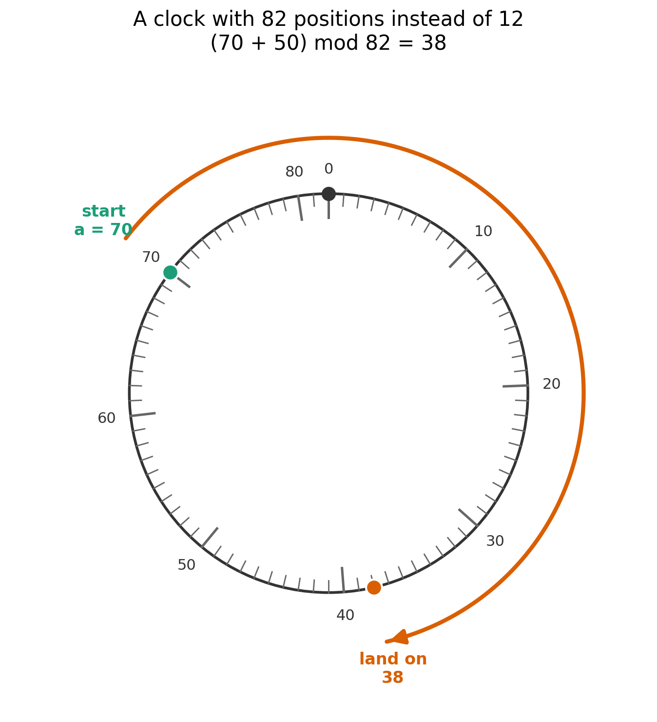
There are 82 x 82 = 6,724 possible (a, b) pairs. I generated all of them, shuffled, and split 50/50. The model never sees the correct answer for the held-out half during training. The only way it scores well there is by inferring the actual rule, not by pattern-matching against problems it's already seen.

The model

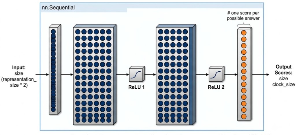
I build a small model with two layers and an embedding table.

class ClockMathBrain(nn.Module):
    def __init__(self, clock_size, representation_size):
        super().__init__()
        self.number_to_representation = nn.Embedding(clock_size, representation_size)
        self.mixer = nn.Sequential(
            nn.Linear(representation_size * 2, representation_size * 4),
            nn.ReLU(),
            nn.Linear(representation_size * 4, representation_size * 4),
            nn.ReLU(),
            nn.Linear(representation_size * 4, clock_size),
        )

    def forward(self, a, b):
        representation = torch.cat(
            [self.number_to_representation(a), self.number_to_representation(b)],
            dim=-1,
        )
        return self.mixer(representation)

Each number from 0 to 81 gets its own 128-dimensional embedding. The embeddings for a and b are concatenated and pushed through the Multilayer Perceptron, which outputs a score for each of the 82 possible answers. I used ReLU as activation function between the layers, since is the most common used nowadays.

At every step, the loss tells you which way each weight should move to make the model a little less wrong. The optimizer is the rule for turning that direction into an actual step aka how far to move each weight, right now. Plain gradient descent moves every weight by the same fixed-size step. AdamW, the optimizer I used here, is a bit smarter about it. It looks at how consistent each weight's updates have been lately, so a weight that keeps getting pushed the same way, step after step, gets a bigger, more confident move, and one whose direction keeps flip-flopping gets a smaller, more cautious one. Every weight ends up with its own effective step size instead of one number shared across the whole network.

optimizer = torch.optim.AdamW(
    model.parameters(),
    lr=1e-3,
    weight_decay=1.0,   # <- this is the setting the whole post is about
    betas=(0.9, 0.98),
)

def score(idx):
    """What fraction of these problems does the model currently get right?"""
    model.eval()
    with torch.no_grad():
        guesses = model(a[idx], b[idx]).argmax(dim=-1)
        return (guesses == answer[idx]).float().mean().item()

def current_parameter_l2_norm():
    """How big are all the model's parameters combined?"""
    return sum(param.norm().item() ** 2 for param in model.parameters()) ** 0.5

The optimizer above is what actually shrinks the model as it trains, AdamW doesn't add anything to the loss, it applies weight decay directly to the weights, on top of the normal gradient-based update. At every step, every parameter gets pulled down by an extra lr * weight_decay * param, no matter what the loss gradient says. That's different from old-school L2 regularization, where you'd add a penalty term to the loss itself and let the gradient do the shrinking. Here the shrinking is decoupled, it happens as its own separate step, every single time, whether the loss cares or not.

That distinction matters once the model has memorized the practice set. Once the practice loss hits zero, the gradient has nothing left to push against, it stops trying to change the weights. The decay term doesn't know or care that the loss is happy. It keeps subtracting a little from every weight, step after step, which is why the weights keep shrinking for thousands of steps after the practice score is already sitting at a perfect 1.00.

weight_decay=1.0 is a lot. Production models usually sit somewhere around 0.01 to 0.1. I turned it up here so the shrinking would clearly beat the memorized solution within a few thousand steps rather than needing a run too long to be worth doing.

The current_parameter_l2_norm is for telling how big all the weights are combined, computed with the same formula used in L2 regularization:

$$\text{parameter L2 norm} = \sqrt{\sum_i \|W_i\|_2^2}$$

where each $W_i$ is one weight or bias tensor in the model.

I trained for 3,000 steps, checking the practice score and the parameter L2 norm every 100 steps.

Steps 0-100: memorization. Practice score hits 1.00 almost immediately. Quiz score sits at 0.00. Classic overfitting: the model is looking up answers, not deriving them.

Steps 100-1,200: the plateau. Practice score stays pinned at 1.00. Quiz score doesn't move. If you stopped training here, you'd conclude the model had learned nothing generalizable and call it a day. Twelve hundred steps of watching a flat line is exactly why grokking is easy to miss in ordinary training runs. Nobody waits.

Steps 1,200-2,400: the click. Quiz score breaks from 0.00, and climbs the rest of the way to 1.00 by step 2,400:

I plot the parameter L2 norm under the same timeline:

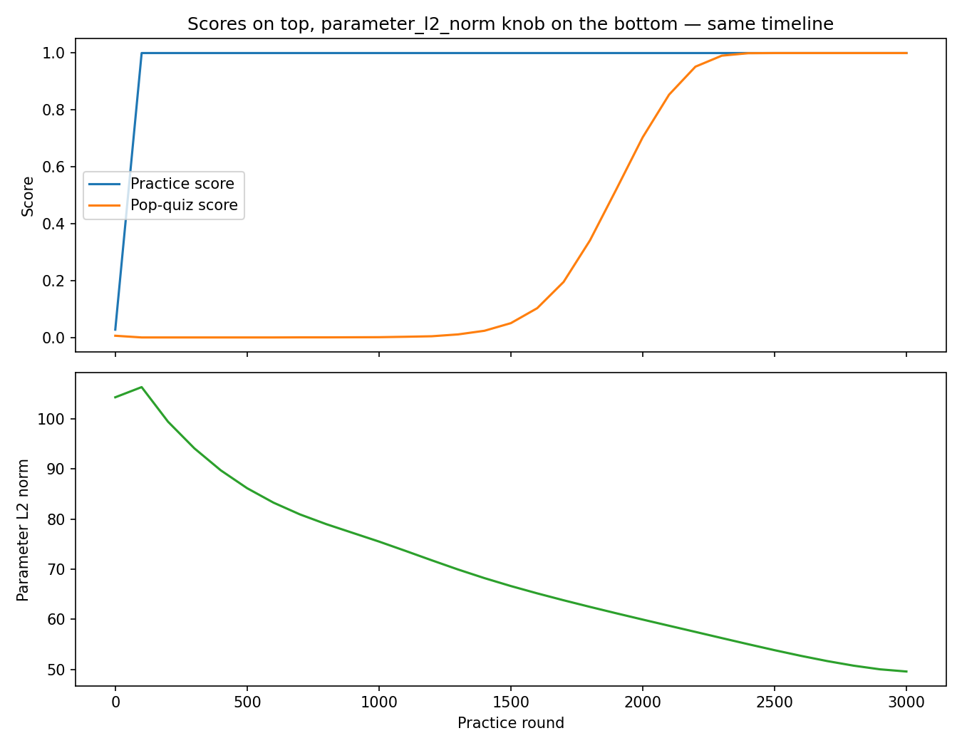
The norm falls the entire time, from about 106 right after memorization to 49.6 by the end. Generalization doesn't happen at some special weight norm value. It happens partway down a smooth, monotonic decline.

I tested withweight_decay=0.0 and retrained from scratch with the same architecture, problem, number of steps etc, to compare, only the weight decay coefficient changed.

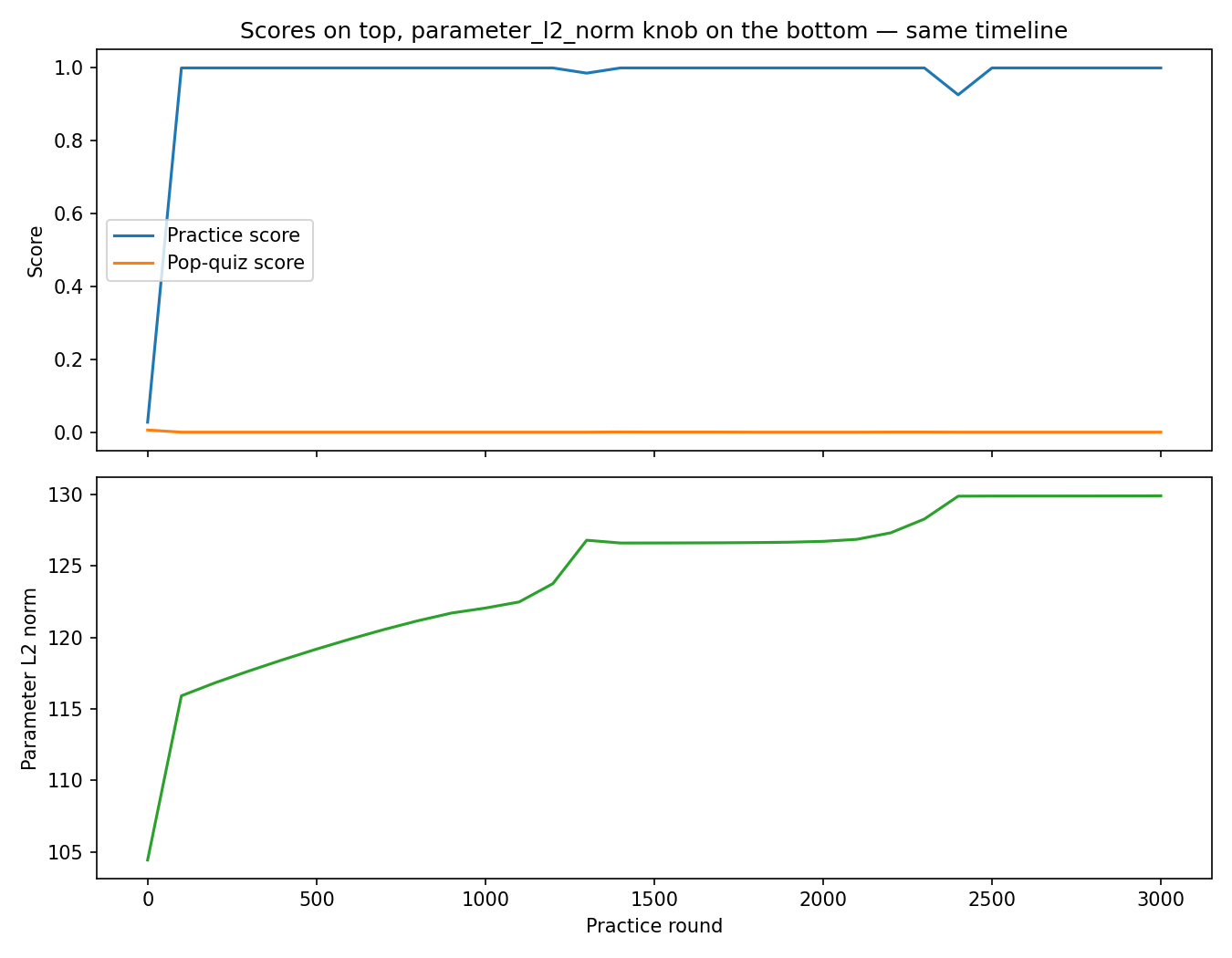
The model as you see in the orange line never generalized on anything, and since there is no penalty for the weights size the L2 norm increased from 104 to 130, practically making the model overfit even more the train set. Without the constraint pulling the norm down, the model has no pressure to find the smaller, simpler solution that happens to generalize. It just gets better and better at memorizing.

An 82-element addition table is silly on its own, I just did it for fun in order to learn something, at the end of the day nobody needs a neural network to compute modular arithmetic. The reason this is worth building is that the same instant memorization, a long flat stretch, then a sudden jump to generalization, has been observed in training runs on much larger, real models and something that worths keeping in mind.