Finding a book through Reinforcement Learning

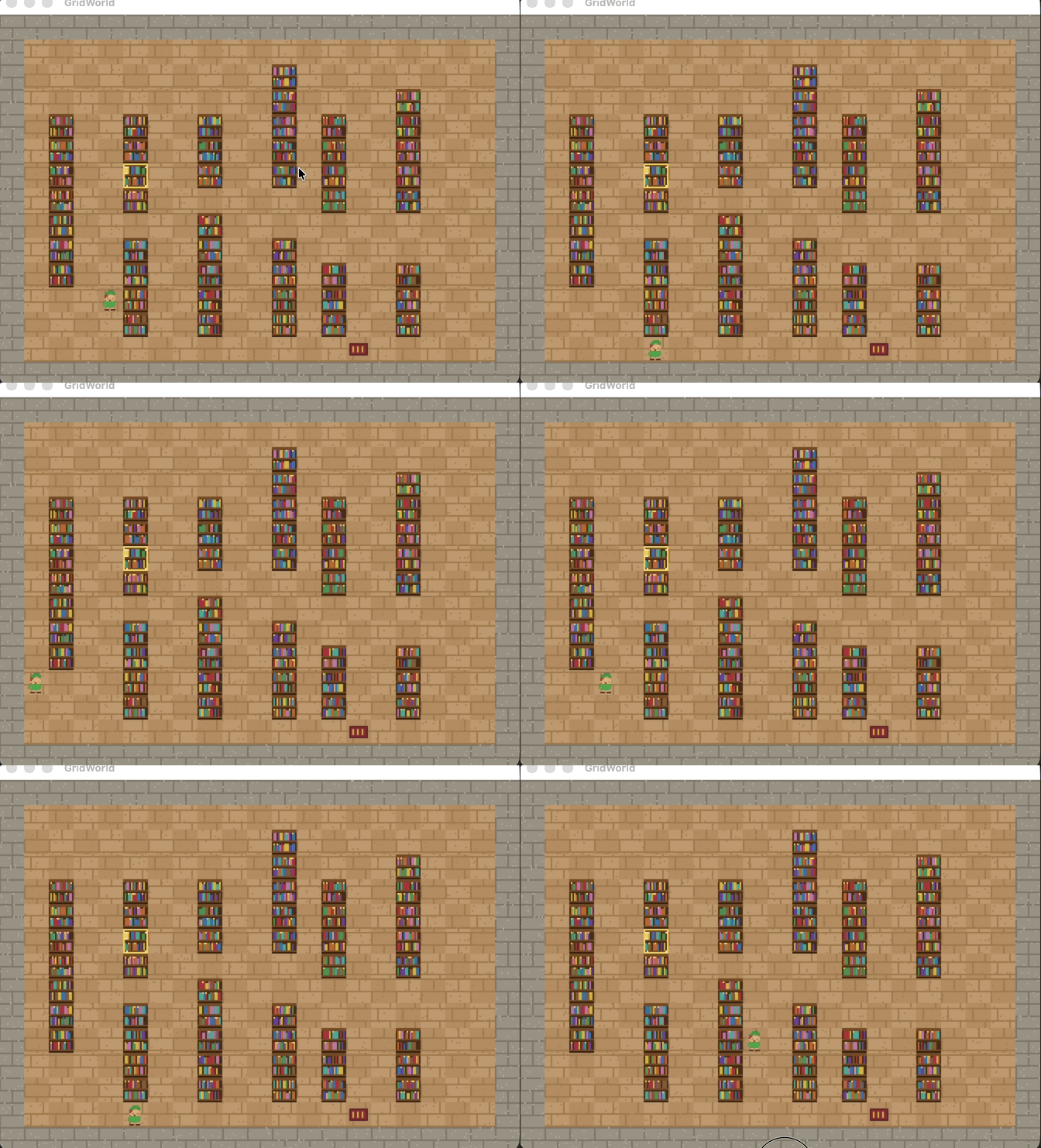
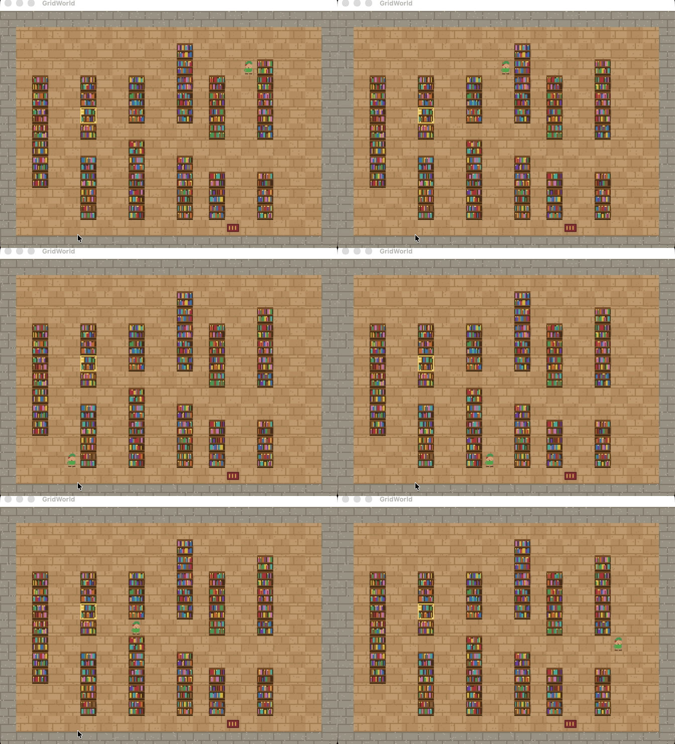
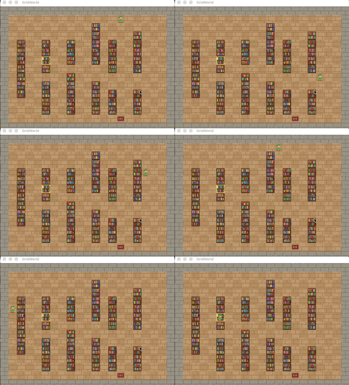
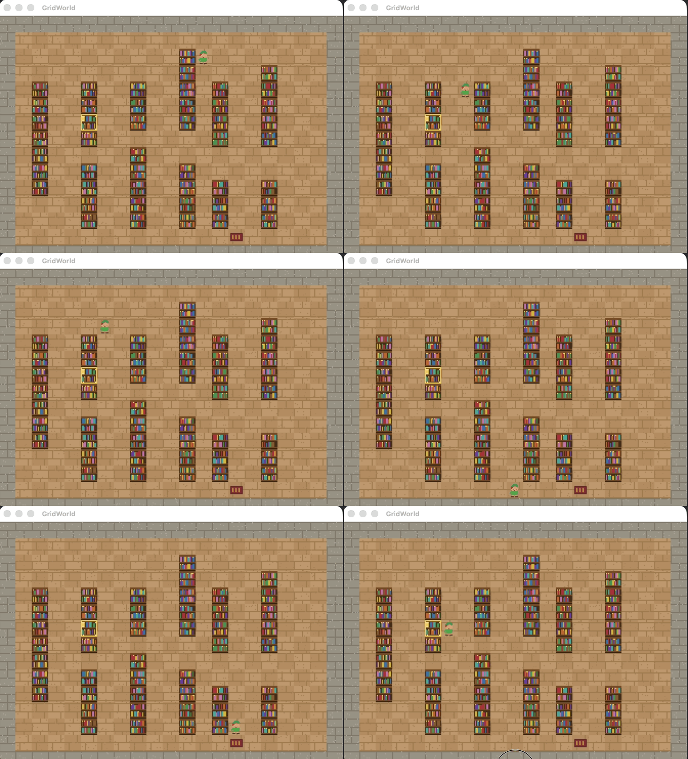
Lately I was studying some fundamental reinforcement learning algorithms, and as I was sitting in the library in Schöneberg I was thinking about what I could implement to see them in practice. The idea that came to me was a small example where an agent tries to find a book in a bookshelf. So I built a small gridworld, a procedurally generated library with some rows of shelves, one door in, one book somewhere in the stacks and the goal being to find the book. I wanted something small enough to show me what the trade-offs actually look like instead of just reading about them.

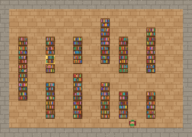
I was reading "Grokking Deep Reinforcement Learning" at the time, so the algorithms I picked came from the book, mainly model-free ones. Model-free means the agent doesn't know the rules of the environment in advance: no transition probabilities, no map of the obstacles, no reward function. What it does instead is visit a tile and think "I did this, I ended up here, I got this reward". It builds a value estimate purely from that stream of experiences. The algorithms differ almost entirely in one thing: how much of that stream to trust before updating anything.

Instead of just tracking a reward, I tracked how many steps above optimal a policy takes. Zero means it found the actual shortest path.

Every algorithm below explores the same way, with epsilon-greedy: most of the time the agent takes the current best action it knows about, and with a small probability ε it picks one at random. That random pick is what I call a wander further down.

Monte Carlo

Monte Carlo (MC) methods estimate values by averaging the actual discounted return from complete episodes, not a guess about what happens next. One episode looks like this:

1. From the door, pick actions with epsilon-greedy: usually the current best, sometimes random. Walk until you find the book (or the episode is cut off). Store every (tile, action, reward) along the way.
2. Starting from the last step and walking backward, compute the actual discounted return that followed each visit: the rewards you really got from that point to the end of the episode. No bootstrap.
3. Nudge Q(tile, action) a little toward that return, for every visit.
4. Repeat for the next episode. Nothing inside an episode gets corrected until the episode is over.

It's the slowest and noisiest method here. One unusually long or short episode swings every value visited along the way.

Here it is running in the library:

Three ways to bootstrap after a single step

Bootstrapping means updating a value using another estimated value, instead of waiting for the real outcome. Monte Carlo never does this. The agent has to find the book (or the episode has to end) before any of the steps it took get an update, and that update is the actual discounted return, not a guess about what happens next. One-step methods skip the wait. After a single move they look at the value they already have for the next state-action and treat that number as the rest of the return.

SARSA, Expected SARSA, and Q-learning all update after one real step instead of waiting for the episode to end. The only thing separating them is what each one bootstraps off, which is to say what it guesses with.

SARSA uses the value of whatever action the agent is actually about to take next. One step looks like this:

1. From the current tile, pick an action with epsilon-greedy: usually the current best, sometimes random.
2. Take that step. Observe the reward and the tile you land on.
3. From the new tile, pick the next action the same way, epsilon-greedy. This is the action you are actually about to take, wander and all. The target is that reward plus the discounted Q-value of (new tile, next action).
4. Nudge Q(tile you left, action you took) a little toward that target.
5. Repeat from the new tile and the next action you already picked, until the book is found or the episode ends.

It's on-policy: it learns the value of its own real, exploring, occasionally-wrong behavior.

Expected SARSA uses the average value over every action, weighted by how likely epsilon-greedy is to pick each one. One step looks like this:

1. From the current tile, pick an action with epsilon-greedy: usually the current best, sometimes random.
2. Take that step. Observe the reward and the tile you land on.
3. From the new tile, do not pick one next action for the update. Average every possible next action's Q-value, weighted by the chance epsilon-greedy would pick each one: almost all the mass on the current best, a little on every action including the wander. The target is that reward plus the discounted average.
4. Nudge Q(tile you left, action you took) a little toward that target.
5. Repeat from the new tile until the book is found or the episode ends.

Same on-policy spirit, but it removes "which random action happened to get rolled" from the target entirely, which lowers variance and usually makes it a smoother learner than plain SARSA.

Q-learning uses the value of the best action available, regardless of what the agent actually does next. One step looks like this:

1. From the current tile, pick an action with epsilon-greedy: usually the current best, sometimes random.
2. Take that step. Observe the reward and the tile you land on.
3. From the new tile, look at every possible next action and take the highest Q-value among them. The target is that reward plus the discounted max.
4. Nudge Q(tile you left, action you took) a little toward that target.
5. Repeat from the new tile until the book is found or the episode ends.

The action you took can be a wander. The action you bootstrap off is always the current best. That's the off-policy choice: the target reflects an idealized greedy policy, not whatever the agent actually stumbles into while exploring. It's the fearless one of the three, because its value estimate never has to account for the chance that the agent slips.

The dial between one step and the whole episode

n-step SARSA sits in the gap between Monte Carlo and one-step SARSA by looking ahead a fixed number of real steps (three, here) before bootstrapping. One update looks like this:

1. Walk with epsilon-greedy, one tile at a time, same as SARSA. Keep a short memory of the last three (tile, action, reward).
2. Once three real rewards are in hand, look at the oldest (tile, action) in that memory.
3. The target is those three rewards, discounted, plus the discounted Q of (tile you're on now, action you're about to take). That last term is the bootstrap, same as SARSA, just three steps later.
4. Nudge that oldest Q a little toward that target.
5. Slide the memory forward one step and repeat. When the episode ends, flush whatever is still in memory using the remaining real return, with no bootstrap.

Think of it as a dial: more real signal per update, at the cost of a delayed, choppier one, since nothing about a state can be written until n steps later.

n-step Q-learning is the same three-step window, with Q-learning's max at the far end. One update looks like this:

1. Walk with epsilon-greedy, one tile at a time. Keep a short memory of the last three (tile, action, reward).
2. Once three real rewards are in hand, look at the oldest (tile, action) in that memory.
3. The target is those three rewards, discounted, plus the discounted max Q over every action from the tile you're on now. Ignore whatever you are actually about to do next.
4. Nudge that oldest Q a little toward that target.
5. Slide the memory forward one step and repeat. When the episode ends, flush with the remaining real return, no bootstrap.

SARSA(λ) chases the same multi-step goal without a hard cutoff. It keeps a decaying eligibility trace over every recently visited state-action pair and spreads each step's error across all of them at once. One step looks like this:

1. From the current tile, pick an action with epsilon-greedy (or reuse the one you already picked, same as SARSA). Take that step. Observe the reward and the tile you land on.
2. From the new tile, pick the next action the same way. The error is that reward plus discounted Q(new tile, next action), minus Q(tile you left, action you took).
3. Bump the eligibility of (tile you left, action you took). Pairs you visited recently still have some eligibility left.
4. Nudge every (tile, action) a little toward that error, scaled by how eligible each one is. Then decay every eligibility.
5. Repeat from the new tile and the next action you already picked, until the book is found or the episode ends.

Q(λ) is the same trace machinery with Q-learning's max, plus one extra check, because the target is off-policy. One step looks like this:

1. From the current tile, pick an action with epsilon-greedy. Take that step. Observe the reward and the tile you land on.
2. From the new tile, take the highest Q-value among every possible next action. The error is that reward plus the discounted max, minus Q(tile you left, action you took).
3. Bump the eligibility of (tile you left, action you took). Nudge every (tile, action) toward that error, scaled by eligibility.
4. Pick the next action you will actually take, epsilon-greedy.
5. If that next action is the greedy one, decay every eligibility and continue. If it is a wander, reset every eligibility to zero. The trace's whole premise was "this was a run of the greedy policy," and an exploratory step makes that stop being true. Repeat from the new tile.

Two targeted fixes

Double Q-learning patches a specific, well-documented flaw in Q-learning: taking a max over noisy estimates is a biased estimator of the true max, so Q-learning tends to learn values that are a little too optimistic. The fix is two tables instead of one. One step looks like this:

1. Keep two Q tables. From the current tile, pick an action with epsilon-greedy over both of them combined (their sum).
2. Take that step. Observe the reward and the tile you land on.
3. Flip a coin. Suppose it says update table A: from the new tile, pick the best action according to table A, but read that action's value from table B. The target is the reward plus that discounted value from B.
4. Nudge table A's Q(tile you left, action you took) a little toward that target. Table B is left alone this step.
5. Repeat from the new tile. Next time the coin might update B, using A as the evaluator.

A noisy overestimate in A never gets to vouch for itself.

Dyna-Q takes a completely different angle. It remembers every (state, action) → (reward, next state) transition it has seen and replays a batch of them as extra Q-learning updates between real steps. One step looks like this:

1. From the current tile, pick an action with epsilon-greedy. Take that step. Observe the reward and the tile you land on.
2. Do a Q-learning update on that real transition: the target is the reward plus the discounted max Q from the new tile. Nudge Q(tile you left, action you took) toward it.
3. Remember the transition: (tile, action) maps to (reward, next tile). The library is deterministic, so one memory is the whole model.
4. Then, without walking anywhere, replay a batch of remembered transitions. For each one, do the same Q-learning update as if you had just taken that step again.
5. Repeat from the new tile.

That squeezes more learning out of experience it's already spent, with no new interaction with the environment required. It assumes the world is deterministic, which this library is, so it's exactly the setup where the trick should pay off.

And with replay switched on:

The race

Four algorithms, one per family, same library, same 3,000 episodes, ten independent training runs averaged: Monte Carlo (no bootstrap), SARSA (on-policy, one step), Q-learning (off-policy, one step), Dyna-Q (off-policy plus replay).

Dyna-Q is essentially walking the optimal 16-step path by episode 50 and stays there for the rest of training. The extra replayed updates do what the theory promises: they squeeze more value out of each real episode than the episode alone would give. Q-learning isn't far behind, settling in by around episode 100. Both are functionally done learning before Monte Carlo has even had 100 real episodes to work with.

Monte Carlo and SARSA tell a noisier story. Monte Carlo needs on the order of 2,000 episodes before its policy is reliably near-optimal, and even in its last 500 training episodes it still fails to reach the book outright about 5% of the time. Full-episode returns are an honest signal, but a slow and high-variance one. SARSA settles faster than Monte Carlo, by roughly episode 1,100, but never fully stops flickering either: about 3% of its late-training rollouts still miss completely, which is what those repeated spikes near the end of the chart are. That's not noise from too few training seeds. It's a fixed, never-decaying epsilon at work: SARSA is learning the value of a policy that keeps exploring forever, so its target keeps a small amount of that exploration risk priced in, permanently.

The full picture

Two results here surprised me enough that I reran them before trusting the numbers. First, Q(λ) lands in the same fast-and-rock-solid tier as plain Q-learning, Double Q-learning, and Dyna-Q: optimal by episode 25, with zero instability afterward. That's a clean confirmation that Watkins's trace-reset trick (drop all accumulated credit the instant the agent takes an exploratory action) works. An off-policy method with eligibility traces bolted on loses none of Q-learning's reliability.

Second, and more surprising: n-step SARSA and SARSA(λ) are the two worst performers in the entire comparison, worse than plain one-step SARSA, not better. Neither ever satisfies a "stayed under one step off optimal for ten straight checkpoints" bar within 3,000 episodes. Late in training, n-step SARSA settles around 237 steps off optimal and SARSA(λ) around 199. On paper both are supposed to be strict improvements on one-step SARSA: more real signal per update, faster credit assignment. In practice, on this task, with a fixed epsilon that never decays, spreading a noisy on-policy target across a 3-step window or a decaying trace seems to spread the noise just as effectively as it spreads the signal. One bad exploratory step now contaminates several state-action pairs' estimates instead of just one. n-step Q-learning and Q(λ) don't have this problem nearly as badly, which points at the mechanism. Multi-step methods aren't noisy by themselves. They amplify whatever noise is already in the target, and only the on-policy target has that noise built in.

What I'd actually reach for

If I had to pick one algorithm for a small, fully-observable, deterministic task like this, it's Dyna-Q: fastest to a reliable policy, no caveats anywhere in the data. But the more useful thing this comparison taught me isn't which one wins. It's that the on-policy/off-policy line matters more than the one-step/multi-step line. Every off-policy method here (Q-learning, Q(λ), Double Q-learning, Dyna-Q) converged fast and stayed converged. Every on-policy method (SARSA and both of its more sophisticated multi-step descendants) stayed genuinely noisy for the entire run, and the "smarter" versions of it were noisier still, not less. If exploration never decays, on-policy control never fully lets go of that decision, no matter how many steps or how much trace you stack on top of it.